This post is a summary of lectures 6 to 8 (Videos 17 to 25) of Stanford CS224W, ‘Machine Learning with Graphs’ course. (youtube)
Introduction to Graph Neural Networks
The goal is to find an encoding of vector $v$ based graph structure
$$ ENC(v) = \text{Multiple layers of non-linear transformation} \ \text{based on graph structure} $$
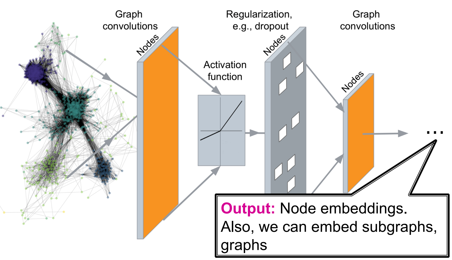
Tasks
- Node classification
- Link prediction
- Community detection
- Network similarity
😐 Modern deep learning toolbox is designed for simple sequences and grids
But graphs:
- Arbitrary size and complex topological structure
- No Fixed ordering or reference point
- Often dynamic and have multimodal features
Basic of Deep Learning
I skip this lecture.
Deep Learning for Graphs
| Notion | Description |
|---|---|
| $G$ | Graph |
| $V$ | Vertex set |
| $A$ | Adjacency matrix |
| $X\in \mathbb{R}^{m\times|V|}$ | Matrix of node features |
| $v\in V$ | A node |
| $N(v)$ | Set of neighbors of $v$ |
Naive approach
Join adjacency matrix and feature and then feed them to the deep neural net:

- $O(|V|)$ parameters
- Not applicable to graphs with different size
- Depends on node ordering
CNNs similar idea
💡Transform information at the neighbors and combine it.
- Transform messages $h_i$ from neighbors: $W_ih_i$
- Add them up: $\sum_iW_ih_i$
Graph Convolutional Neural Network (GCN)
💡Network neighborhood defines a computation graph
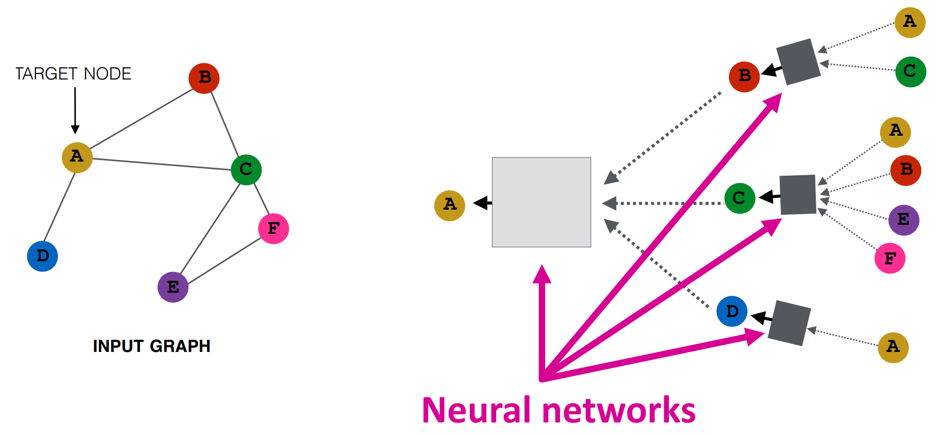
The math
- Initial 0th layer embeddings are equal to node feature
$$h_v^0=x_v$$
- For each layer
$$ h_v^{(l+1)} = \textcolor{orange}{\sigma}( \textcolor{pink}{W_l} \textcolor{skyblue}{\sum_{u\in N(v)}\frac{h_u^{(l)}}{|N(v)|}} + \textcolor{pink}{B_l}h_v ), \quad \forall l \in \lbrace 0, \dots, \textcolor{purple}{L}-1 \rbrace $$
- Where:
- $\textcolor{orange}{\sigma}$: None-linearity (e.g. ReLU)
- $\textcolor{pink}{W_l}$, $\textcolor{pink}{B_l}$: Trainable weight matrix
- $\textcolor{skyblue}{\sum_{u\in N(v)}\frac{h_u^{(l)}}{|N(v)|}}$: Averages of neighbor’s previous layer embeddings
- $\textcolor{purple}{L}$: Total number of layers
- Embedding after L layers of neighborhood aggregation $$z_v=h_v^{(L)}$$
Matrix formulation
- $H^{(l)}=[h_1^{(l)}\dots h_{|V|}^{(l)}]^T$
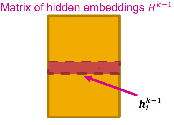
- $\sum_{u\in N(v)} h_u^{(l)} = A_{v,:}H^{(l)}$
- $A_{v,:}$ means row $v$ of adjacency matrix $A$
- $D$ is diagonal matrix where: $D_{v,v}=\text{Deg}(v) + \epsilon
$
- $D_{v,v}^{-1}=1/(|N(v)|+\epsilon)$
- $\epsilon$ prevents dividing by zero.
- $\tilde{A}=D^{-1}A$
Matrix form
$$ H^{(l+1)}=\sigma(\textcolor{tomato}{\tilde{A}H^{(l)}W_l^T } + \textcolor{aqua}{H^{(l)}B_l^T}) $$
- Neighborhood aggregation
- Self transformation
🙃 Not all GNNs can be expressed in matrix form, when aggregation function is complex.
How to train a GNN
Supervised
Minimize loss between GNN output and label
$$ \min_{\theta}\mathcal{L}(y,f(z_v)) $$
Unsupervised
Because no label is available, use the graph structure as the supervision (e.g. node similarity based random walks, matrix factorization, etc.).
Inductive capacity
The same aggregation parameters are shared for all nodes
- The number of model parameters is sublinear in $|V|$
- Generalize to unseen nodes
A General GNN Framework
Each topic will be discussed in next sections
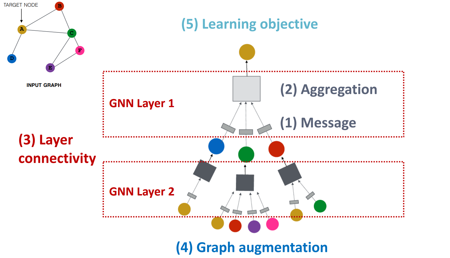
GNN Layer = Message + Aggregation
- Different instantiation under this perspective
- GCN, GraphSAGE, GAT, …
Layer Connectivity
- Stack layers sequentially
- Ways of adding skip connection
Graph Augmentation
- Graph feature augmentation
- Graph structure augmentation
Learning Objective
- Supervised/Unsupervised objectives
- Node/Edge/Graph level objectives
A Single Layer of GNN
Message + Aggregation Framework
Message
$$ m_u^{(l)} = \text{MSG}^{(l)}(h_u^{(l-1)}), \quad u\in \lbrace N(v) \cup v \rbrace $$
Example: A linear layer $m_u^{(l)}=W^{(l)}h_u^{(l-1)}$
✍️ Note: Usually a different message computation is for neighbors and node $v$ itself. example:
- $m_u^{(l)}=\textcolor{tomato}{W^{(l)}}h_u^{(l)}$
- $m_v^{(l)}=\textcolor{dodgerblue}{B^{(l)}}h_v^{(l)}$
Aggregation
$$ h_v^{(l)} = \text{AGG}^{(l)}(\lbrace m_u^{l}, u \in N(v) \rbrace, m_v^{(l)}) $$
⚠️ $\text{AGG}^{(l)}$ should be an order invariant function (works on sets/multi-sets, not sequences)
Example: Sum(.), Mean(.), Max(.), etc.
- Pooling ones (like Max) are coordinate-wise.
✍️ Note: We can (should!) Add expressiveness using Nonlinearity
- $\sigma(\cdot)$: $\text{Sigmoid}(\cdot)$, $\text{ReLU}(\cdot)$, etc.
- Can be added to message or aggregation
⬇️ In the followings deepppink is message and orange is aggregation.
GCN
$$ h_v^{(l)} = \textcolor{orange}{\sigma( \sum_{u\in N(v)}} \textcolor{deeppink}{W^{(l)}\frac{h_u^{(l)}}{|N(v)|}} \textcolor{orange}{)} $$
✍️ In the GCN original paper they used different normalization rather than $1/|N(v)|$, link.
GraphSAGE
$$ h_v^{(l)} = \textcolor{orange}{\sigma( W^{(l)}\cdot \text{CONCAT(}} \textcolor{deeppink}{h_v^{(l-1)}}, \textcolor{orange}{\text{AGG}(} \lbrace\textcolor{deeppink}{h_u^{(l-1)}}, \forall u \in N(v)\rbrace \textcolor{orange}{)))} $$
✍️ Notes:
- Two-stage aggregation is used:
- Aggregation from node neighbors
- the output of this stage is a message itself
- Further aggregation from the node itself
- Aggregation from node neighbors
- $\text{AGG}$ can be Mean, Pool, or apply LSTM to reshuffled of neighbors.
- (Optional) $l_2$ Normalization
- $h_v^{(l)} \leftarrow h_v^{(l)}/||h_v^{(l)} ||_2$
- In some cases results in performance improvement
GAT (Graph ATtention)
$$ h_v^{(l)} = \textcolor{orange}{\sigma( \sum_{u\in N(v)}} \textcolor{deeppink}{\alpha_{vu}W_V^{(l)}h_u^{(l-1)}} \textcolor{orange}{)} $$
Where:
- Attention coefficient $e_{vu}$ (indicates importance of $u$’s message to node $v$)
$$ e_{vu} = a(W_Q^{(l)}h_v^{(l-1)},W_K^{(l)}h_u^{(l-1)}) $$
- Normalize $e_{vu}$ to get attention weight $\alpha_{vu}$ (using softmax)
$$ \alpha_{vu} = \frac{\text{exp}(e_{vu})}{\sum_{k\in N(v)}\text{exp}{(e_{vk})}} $$
✍️ Notes:
- Attention is inspired by cognitive attention
- In GCN/GraphSAGE: $\alpha_{vu}=1/|N(v)|$
- $a$ can be a simple single-layer neural network
- In attention terminology, $K$ is key, $Q$ is query, and $V$ is value.
Multi-head attention
- Create multiple attention score
- $h_v^{(l)}[1] = \sigma(\sum_{u\in N(v)}\textcolor{red}{\alpha_{vu}^1}W^{(l)}h_u^{(l-1)})$
- $h_v^{(l)}[2] = \sigma(\sum_{u\in N(v)}\textcolor{green}{\alpha_{vu}^2}W^{(l)}h_u^{(l-1)})$
- $h_v^{(l)}[3] = \sigma(\sum_{u\in N(v)}\textcolor{blue}{\alpha_{vu}^3}W^{(l)}h_u^{(l-1)})$
- Aggregate (e.g. concatenation)
- $h_v^{(l)} = \text{AGG}(h_v^{(l)}[1],h_v^{(l)}[2],h_v^{(l)}[3])$
Benefits of attention mechanism
- Computationally efficient
- Storage efficient
- Localized
- Inductive capability
GNN Layer in Practice
Many deep learning techniques can be used here, I just mention a few of them:
- Batch Normalization
- Stabilize neural network training
- Dropout
- Prevent over-fitting
- Attention/Gating
- Control the importance of a message
Stacking Multiple Layers of GNNs
Over-smoothing problem
After Adding multiple layers of GNNs sequentially, all nodes converge to similar embedding which makes them hard to differentiate. It’s because of the Receptive field overlap in the depth layer.
solution
Graph Augmentation for GNNs
Our assumption so far
Raw input graph = Computation graph
Reasons for breaking this assumption
- Features
- The input graph lacks features
- $\rightarrow$ Feature augmentation
- The input graph lacks features
- Graph structure
- The graph is too sparse
- $\rightarrow$ Add virtual nodes / edges
- The graph is too dense
- $\rightarrow$ Sample neighbors when doing message passing
- The graph is too large
- $\rightarrow$ Sample subgraphs to compute embedding
- The graph is too sparse
Feature augmentation
Used when graph does not have node features (common when we only have adjacency matrix)
Standard approaches
- Constant value
- Unique ID to nodes
- should be converted to one-hot vectors
Comparison
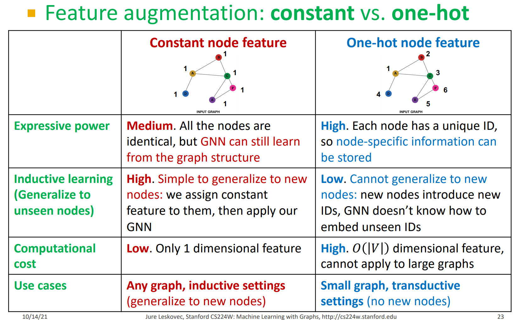
⚠️ Some structures are hard to learn by GNNs
Example: Cycle count feature
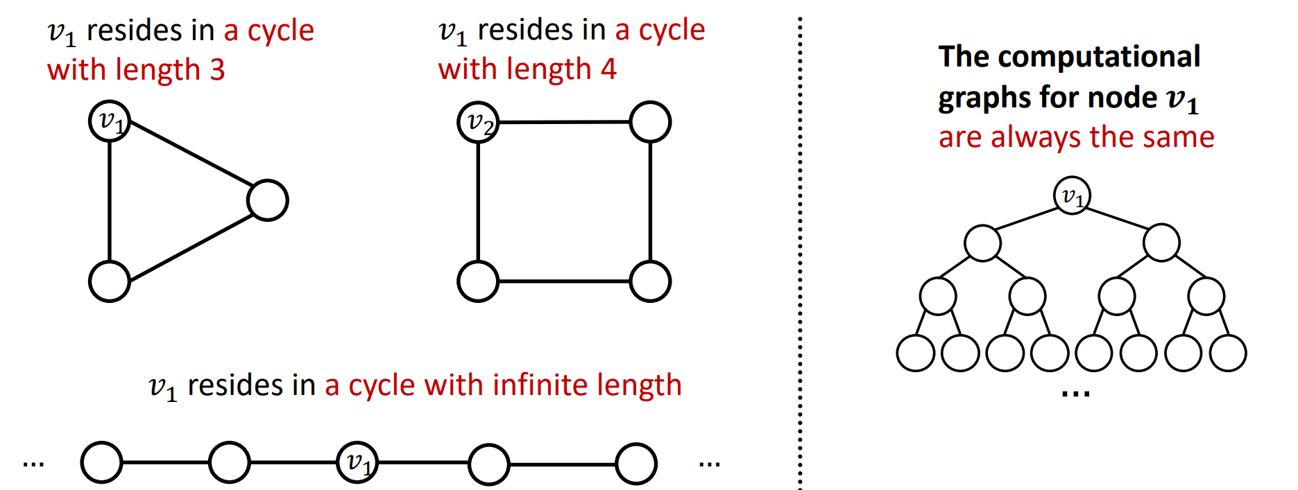
GNN can’t learn the length of a cycle that $v_1$ resides in
Therefore, we should augment node features with cycle count manually by adding a vector of cycle counts like this:
$$ \text{cycle count feature: } [0, 0, 0, 1, 0, 0] $$
where index 0 indicates that $v_1$ resides in cycle of length $0$, index 1 indicates cycle of length $1$, and so on.
Commonly used augmented features
- Node Degree
- PageRank
- Clustering coefficient
- Node centrality
- Eigenvector
- Betweenness
- Closeness
- …
- Graphlet
- …
Add virtual nodes / edges
Virtual edge
Common approach: connect 2-hop neighbors
- instead of using adj. matrix $A$ for GNN computation, use $A^2 + A$
Use cases:
- Bipartite graphs
Virtual node
Add a virtual node and connect it to other nodes (all or some of them)
Benefits:
- Greatly improves message passing in sparse graphs
Node neighborhood sampling
Instead of using all nodes for message passing, (randomly) sample a node’s neighborhood. for example, if a node has 5 neighbors, sample 2 of them in the message passing phase.
Benefits:
- Reduce computational cost
- Allows for scaling to large graphs
- in practice it works great 👌
Prediction with GNNs
GNN training pipeline
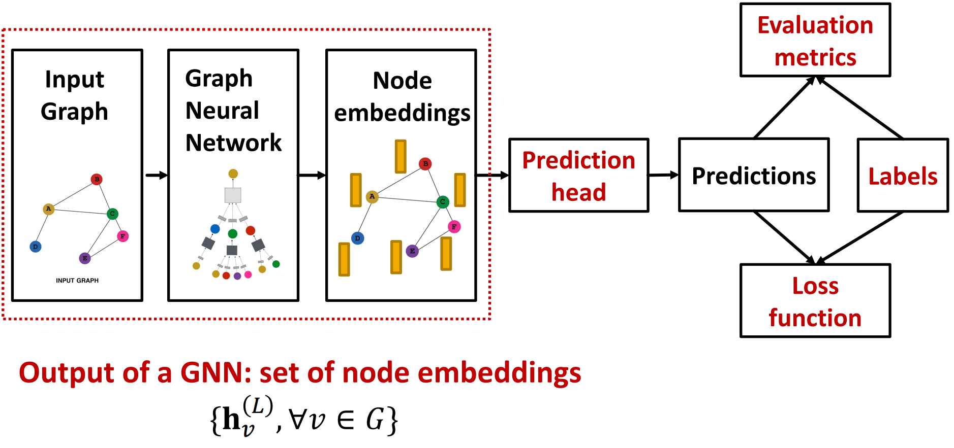
GNN output
GNN output is a set of node embeddings:
$$ \lbrace h_v^{(L)}, \forall v \in G \rbrace $$
Prediction head
- Node-level tasks
- Edge-level tasks
- Graph-level tasks
Node-level
We can directly use node embeddings or transform them into label space ($y_v$ is ground truth label and $\widehat{y}_v$ is model output):
$$ \textcolor{Chartreuse}{\widehat{y}_v = h_v^{(L)}} $$
$$ \text{or} $$
$$ \textcolor{Chartreuse}{\widehat{y}_v = Head_{node}(h_v^{(L)}) = W^{(H)}h_v^{(L)}} $$
Edge-level
$$ \color{Chartreuse} \widehat{y}_{uv} = Head_{edge}(h_u^{(L)},h_v^{(L)}) $$
Options for $Head_{edge}$:
- Concatenation + Linear: $\text{Linear}(\text{Concat}(h_u^{(L)},h_v^{(L)}))$
- Similar to graph attention
- Dot product: $(h_u^{(L)})^T h_v^{(L)}$
- This approach only applies to 1-way prediction
- Applying to $k$-way prediction
- Similar to multi-head attention: $W^{(1)}, …, W^{(K)}$ is trainable
$$ \widehat{y}_{uv}^{(1)} = (h_u^{(L)})^T \textcolor{red}{W^{(1)}}h_v^{(L)} $$
$$ \dots $$
$$ \widehat{y}_{uv}^{(K)} = (h_u^{(L)})^T \textcolor{red}{W^{(K)}}h_v^{(L)} $$
$$ \widehat{y}_{uv} = \text{Concat}(\widehat{y}_{uv}^{(1)}, \dots, \widehat{y}_{uv}^{(K)}) \in \mathbb{R}^k $$
Graph-level
$$ \color{Chartreuse} \widehat{y}_G = Head_{graph}(\lbrace h_v^{(L)} \in \mathbb{R}^d, \forall v \in G \rbrace) $$
Options for $Head_{graph}$:
- Global mean pooling
- Global max pooling
- Global sum pooling
These global pooling methods will work great over small graphs but
⚠️ Global pooling over a (large) graph will lose information
Hierarchical global pooling
Hierarchically pool section of nodes.
Which section?
Diffpool idea:

- Leverage 2 independent GNNs at each level
- GNN A: Compute node embeddings
- GNN B: Compute the cluster that a node belongs to
- GNNs A and B at each level can be executed in parallel
- GNNs A and B are trained jointly
Training GNNs
Setting-up GNN Prediction Tasks
When Things Don’t Go As Planned
The three above topics are almost the same in other deep learning areas so I will put them aside for now.